If you routinely utilize Google Sheets and also ever before require to sum worths with each other based upon some problem in details cells, after that you'll require to understand exactly how to utilize the SUMIF feature in Google Sheets
The capability to sum information with this feature isn't restricted to simply 2 worths. You can sum a whole array. As well as the problem you offer the feature for it to amount or otherwise can rely on several cells in your spread sheet also.

Just How the SUMIF Feature Functions in Google Sheets
SUMIF is a easy spread sheet feature, yet it's adaptable sufficient to ensure that you can do some innovative estimations with it.
You require to mount the feature as complies with:
SUMIF( array, requirement, [sum_range])
The criteria for this feature are as complies with:
- Array: The series of cells you wish to utilize to examine whether to build up the worths.
- Requirement: The problem of the cells you wish to examine.
- Sum_range: This criterion is optional, and also consists of the cells that you wish to amount. If you do not include this criterion, the feature will just summarize the array itself.
The feature shows up easy, yet the reality that you can sum or contrast varieties of several cells permits much more versatility than you might recognize.
A SUMIF Instance with Text
If you prepare to start with the SUMIF feature, the most effective method is to utilize 2 columns in your spread sheet. One column will certainly be for your contrast, and also the various other will certainly be the worths you wish to include.
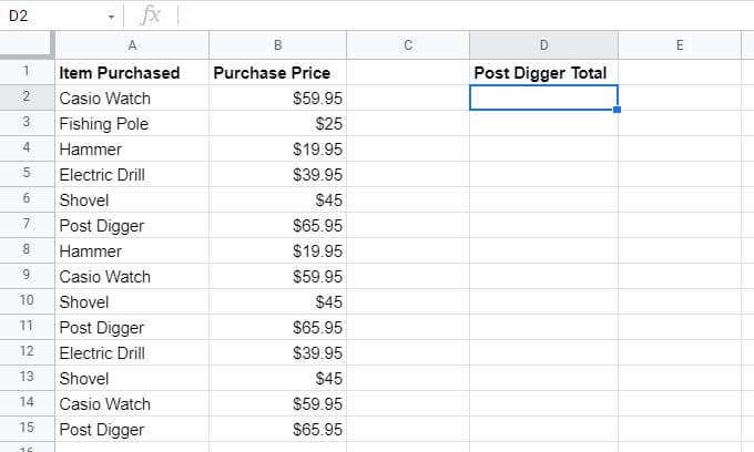
The instance sheet over is that of a shopkeeper that's monitoring acquisitions via a duration. The shopkeeper wishes to produce extra columns that summarize the acquisition costs in column B for details worths in column A.
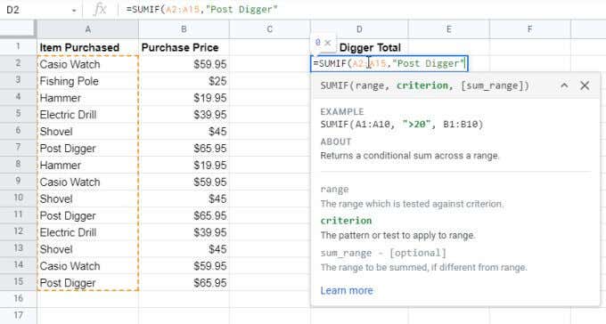
In this situation, the array for contrast would certainly be A2: A15

The requirement would certainly be the keywords for the thing to build up. So, in this situation, to build up every one of the blog post miner acquisitions, the requirement would certainly be the message "Message Miner".
The amount array would certainly be the series of cells with the worths to be summarized. Below, this is B2: B15
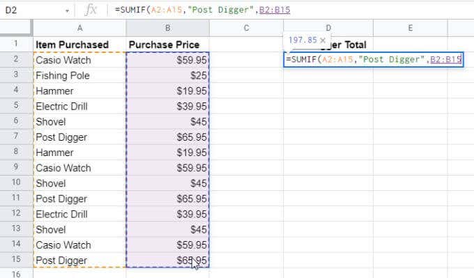
When you push go into, you'll see the details worths from the sum_range column accumulated, yet just with the information from the cells where column A matches the requirement you defined.
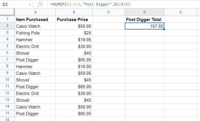
This is an easy method to utilize the SUMIF feature; as a method to tweeze worths out of a 2nd column based upon products noted in the initial.
Note: You do not need to kind the requirement right into the formula inside double-quotes. Rather, you can kind that worth right into a cell in the sheet and also go into that cell right into the formula.
Utilizing SUMIF Operators with Text
While the instance over try to find ideal suits, you can likewise utilize drivers to define components of the message you wish to match. If you change the search standards, you can summarize worths for cells that might not match completely yet offer you with the response you're seeking.
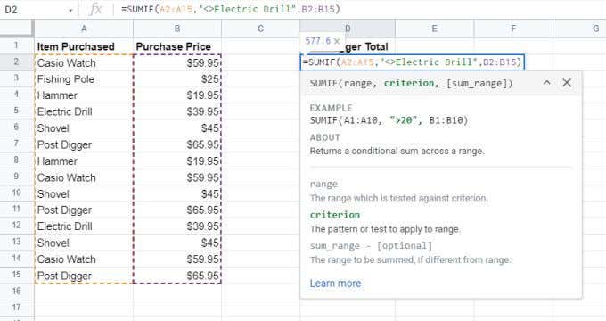
Utilizing the instance over, if you wish to build up acquisitions of all products other than the electrical drill, you will certainly go into the formula the driver.
= SUMIF( A2: A15," Electric Drill", B2: B15)
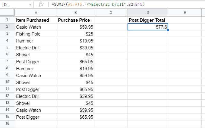
The driver informs the SUMIF feature to overlook "Electric Drill" yet build up all various other products in the B2: B15 array.
As you can see from the outcome listed below, the SUMIF feature works as it should.
You can likewise utilize the complying with drivers when making use of the SUMIF feature with message:
- ?: Look for words with any kind of personality where you've positioned the?. As an example, "S?ovel" will certainly sum any kind of thing beginning with "S" and also finishing with "ovel" with any kind of letter in between.
- *: Look for words that begin or finish with anything. As an example, "* View" will certainly include all products that are any kind of type of watch, no matter brand name.
Note: If you in fact desire the SUMIF feature to look for a personality like "?" or "*" in the message (and also not utilize them as unique personalities), after that beginning those with the tilde personality. As an example, "~?" will consist of the "?" personality in the search message.
Remember that the SUMIF feature is not case-sensitive. So, it does not distinguish in between resources or lower-case letters when you're making use of message as the search standards. This works due to the fact that if the very same word is gotten in with uppercase or without, the SUMIF feature will certainly still identify those as a suit and also will effectively summarize the worths in the worth column.
Utilizing SUMIF Operators with Numbers
Naturally, the SUMIF feature in Google Sheets isn't just beneficial for locating message in columns with connected worths to summarize. You can likewise sum varieties of numbers that fulfill specific problems.
To examine a series of numbers for a problem, you can utilize a collection of contrast drivers.
- >>: Higher Than
- : More than or equivalent to
- : Much less than or equivalent to
- As an example, if you have a checklist of numbers and also you would love to include those over 3000, you would certainly utilize the complying with SUMIF command.= SUMIF( B2: B15, ">> 3000")
Keep in mind that much like with message standards, you do not require to kind the number "3000" right into the formula straight. You can position this number right into a cell and also utilize that cell recommendation rather than "3000" in the formula.
Such As This:
= SUMIF( B2: B15, ">>"&& C2)
One last note prior to we take a look at an instance. You can likewise summarize all worths in a variety that amount to a certain number, simply by not making use of any kind of contrast drivers whatsoever.
SUMIF Instance with Numbers
Allow's take a look at exactly how you can utilize the SUMIF feature in Google Sheets by utilizing a contrast driver with numbers.
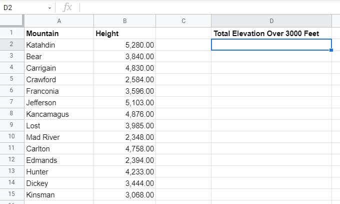
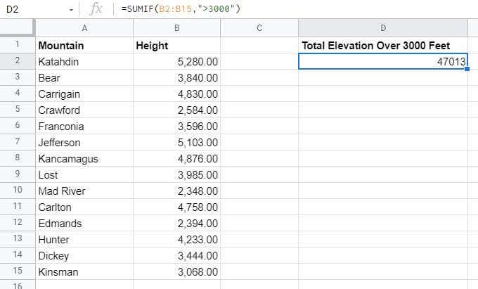
In this instance, picture you're a walker tracking all the hills that you have actually been treking.
In cell D2, you wish to build up the overall elevation of every one of the hills over 3000 feet that you have actually treked.
To do this, you'll require to utilize the formula discussed in the area over.
Press
Go Into
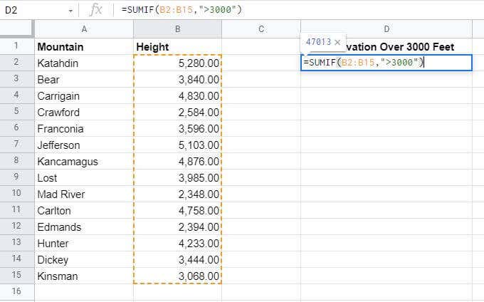
after keying the formula, and also you'll see the lead to this cell. As you can see, the SUMIF feature in Google Sheets summarized all elevation elevations from column B for any kind of hill greater than 3000 feet. The SUMIF formula neglected all worths under that elevation. Utilize the various other conditional drivers noted in the last area to do the very same estimation for numbers much less than, more than or equivalent to, much less than or equivalent to, or equivalent to.
Utilizing SUMIF Operators with Dates
You can likewise utilize the SUMIF feature with days. Once again, the very same contrast drivers noted over use, so you do not need to stress over finding out brand-new ones.
Nonetheless, for the feature to function, days require to be formatted properly in Google Sheets initially.
You can by hand kind the day right into the feature or kind it right into a cell and also recommendation it right into the formula. The layout for this is as complies with:
= SUMIF( B2: B15, ">> 10/4/2019", C2: C15)
Exactly how this functions:
SUMIF will certainly examine the array B2: B15 for any kind of days after 10/4/2019.
If real, SUMIF will certainly summarize any kind of cells in C2: C15 in the very same row where this contrast holds true.
- The resulting total amount will certainly be shown in the cell where you entered the formula.
- If you have a cell where the day isn't formatted by doing this, you can utilize the day feature to reformat the day effectively. As an example, if you have 3 cells (D2, D3, and also D4) that hold the year, month, and also day, you can utilize the complying with formula.
- As an example:
= SUMIF( B2: B15, ">>"&& DAY( D2, D3, D4), C2: C15)
If you have a spread sheet which contains the most recent acquisitions on top of the sheet, you can just utilize the TODAY feature to just summarize today's acquisitions and also overlook the remainder.
= SUMIF( B2: B15, TODAY())
SUMIF in Google Sheets is Straightforward However Versatile
As you can see, the SUMIF formula in Google Sheets does not take a long period of time to find out. However the different means you can utilize it make it so functional.